GEODESICFILT_BASE - Base function for GEODESICFILT.
Contents
Syntax
   F = GEODESICFILT_BASE(I, method, iter, wei, winsize, a, ...
                       rho, sigma, der, int, samp, eign);
See also
Ressembles: GEODESICFILT, ADAPTIVEFILT_BASE, TENSANIFILT_BASE, TENSCALEDIRFILT_BASE, MDLFILT_BASE, CONVOLUTION_BASE, FMMISOPROPAGATION, FMMANISOPROPAGATION, FMM_BASE, PDEM. Requires: POTENTIAL2FRONT, IM2POTENTIAL, WEIGHTFILT_BASE.
Function implementation
function F = geodesicfilt_base(I, method, iter, wei, winsize, a, rho, sigma, ...
    der, int, samp, eign)
checking/setting parameters
% we also accept variable number of inputs
if nargin<=11
    eign = 'zen';
    if nargin<=10,
        samp = 1;
        if nargin<=9
            int = 'fast';
            if nargin<=8,  der = 'fast';  end
        end
    end
end
consider the iterative application of the algorithm
if iter>1
    F = I;
    for i=1:iter
        F = geodesicfilt_base(F, method, wei, winsize, rho, sigma, ...
            a, 1, der, int, samp, eign);
    end
    return
end
internal parameters
[X,Y,C] = size(I);

% the window of analysis: should be odd
winsize = round( (winsize-1)/2 )*2 + 1;
% center of the window
padnum = (winsize-1)/2;
% padnum = max([(winsize-1)/2 ceil(3*sigma) ceil(3*rho)])

% padd the original image for convenient processing
A = padarray(I,[padnum padnum],'replicate','both');

% create the output filtered image
F = zeros(size(I));

% over each local window, the value of the central pixel is estimated; it is
% also used as the starting point for local propagation
start_pt = [padnum+1;padnum+1];
compute once for all the potential function based on the gradient and/or the gradient structure tensor of the multispectral input image and define the propagation function: it is either a scalar field (isotropic case) providing with the speed (strenght) for the propagation (the higher the value at one point, the faster the propagation through this point) or a tensor field (anisotropic case) providing with a speed and a direction for the propagation.
T = im2potential(A, method, a, rho, sigma, der, int, samp, eign);
define the weighting function (see also function WEIGHTFILT_BASE)
if wei==0,     weighting = @wmedweight;
elseif wei>0,  weighting = @gaussweight;
else           weighting = @scaleweight;
end
perform local filtering: FMM is applied locally from the center of the window of analysis in orint to compute local distances from it; those distances are then weightened as to convolve the image locally; the final output value is assigned to the central pixel
estimation on local neighbourhoods
for jj = padnum+1:(padnum+X)
    for kk = padnum+1:(padnum+Y)
        xspan = jj-padnum:jj+padnum;
        yspan = kk-padnum:kk+padnum;

        % compute the matrix defining the metric: the geodesics will follow
        % regions where T is 'large'.
        Dwin = potential2front(T(xspan,yspan,:,:), start_pt);
        % Dwin = Dwin  /max(Dwin(:));

        for i=1:C
            Awin = A(xspan,yspan,i);
%             if i==1&&kk==20 &&jj==20
%                 figure,
%                 subplot(1,2,1), imagesc(rescale(Awin)), colormap gray, axis image
%                 subplot(1,2,2), imagesc(Dwin), colormap gray, axis image
%             end

            F(jj-padnum,kk-padnum,i) = weighting(Awin(:), Dwin(:), wei);
        end
    end

end

% % another way to do it: it uses the already implemented FMM_BASE function,
% % but implies many variable tests at each step of the loop
% for jj = padnum+1:(padnum+1+X-1)
%     for kk = padnum+1:(padnum+1+Y-1)
%         Dwin = fmm_base(T(jj-padnum:jj+padnum,kk-padnum:kk+padnum,:,:), ...
%             'sing', false, start_pt, [], O, [], Inf);
%         for i=1:C
%             Awin = A(jj-padnum:jj+padnum,kk-padnum:kk+padnum,i);
%             F(jj-padnum,kk-padnum,i) = weighting(Awin(:),Dwin(:),p);
%         end
%     end
%
% end
end % end of geodesicfilt_base
Subfunctions
GAUSSWEIGHT - Gaussian-based weighting function
%--------------------------------------------------------------------------
function k = gaussweight(Awin, Dwin, a)
Dwin = exp( - a * Dwin );
t = sum(Dwin);
if(t>0),    Dwin = Dwin/t;  end
k = sum(Awin.*Dwin);

end % end of gaussweight
WMEDWEIGHT - Weighted median-based weighting function. For n
numbers  with positive weights
  (sum of all weights equal to one) the weighted median is defined as the
element
(sum of all weights equal to one) the weighted median is defined as the
element  , such
that:
, such
that: 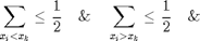
%--------------------------------------------------------------------------
function k = wmedweight(Awin, Dwin)

Dwin = Dwin / max(Dwin(:));

% (line by line) transformation of the input-matrices to line-vectors
d = reshape(Awin',1,[]);
w = reshape(Dwin',1,[]);

% sort the vectors
A = [d' w'];
ASort = sortrows(A,1);

dSort = ASort(:,1)';
wSort = ASort(:,2)';

l = length(wSort);
sumVec = zeros(1,l);    % vector for cumulative sums of the weights
for i = 1:l
    sumVec(i) = sum(wSort(1:i));
end

k = [];     j = 0;

while isempty(k)
    j = j + 1;
    if sumVec(j) >= 0.5
        k = dSort(j);    % value of the weighted median
    end
end

end % end of wmedweight
SCALEWEIGHT - Scale-based weighting function.
%--------------------------------------------------------------------------
function k = scaleweight(Awin, Dwin, a)
Dwin = rescale(Dwin,eps,1) .^ a;
t = sum(Dwin);
if(t>0),    Dwin = Dwin/t;  end
k = sum(Awin.*Dwin);

end % end of scaleweight